Phase 2: Add Obstacle Avoidance

Augment Phase1 to navigate around obstacles and continue CPP. This aims to give full coverage.

Here are the Phase 2 aims:

• Add A-Star (or similar) search algorithm
• Package/Modularize python code and algorithms
• Add tests
• Display visually to monitor how we cover the whole area
• Get this working on the Pi
• Merge CPP and A-Star to give full coverage

A few notes on map representation

There are several different representations we can use for maps. I am going to use Cartesian co-ordinates throughout which is conceptually easy to understand. This means x=left, y=up, just like a normal graph. However, pyhon stores arrays in a different format, compasses use a different frame of reference and matplotlib can also display this data differently. This caused some confusion so I will spell out the differences here:

• Cartesian: Origin (0,0) is bottom left. Tuple (x,y) where x=left/right (column) and y=up/down (rows). All APIs I generate will use this format.
• Python 2D array: Origin (0,0) is top right. Grid indexing is grid[row][col]. So x and y are transposed. Note that row=down, col=right
• Compass: A compass used N=up, E=right. Later on, compass bearings will need to be converted to cartesian and vice-versa.
• If you represent Cartesian in python, you must use y=row and x=col.
• Since python origin is top left, the grid is inverted when using print(grid).
• Matplotlib can be used to display a grid by setting origin='lower' which flips the array back to Cartesian, with origin bottom left.
• The flipping is only on the vertical (y) axis. It is equivalnt to (max_rows -1 -y).
• As this can be very confusing, I am keeping everying in Cartesian and transpose the x and y co-ordinates when storing to python. Matplotlib can be used to display the Cartesian grid. Be aware that print() will show an inverted grid so best use matplotlib for sanity.

Created an A* (A-star) package in the same lib tree structure.

Here is some pseudocode of the approach taken:

import numpy, matplotlib, grid_generation, search_algorithms

grid, resolution = create_grid_with_obstacles()
search_path = generate_cpp_and_astar_path(grid)
plot(grid, search_path)
        

Here is a plot testing A-star only

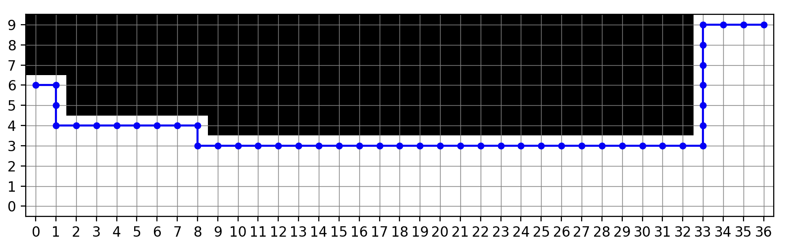
This example gives a starting postion and end position (x,y cartesian co-ordinates) with obstacles in the way. The A-star algorithm successfully works around them.

Here is a plot testing a hybrid (CPP/A-star) solution

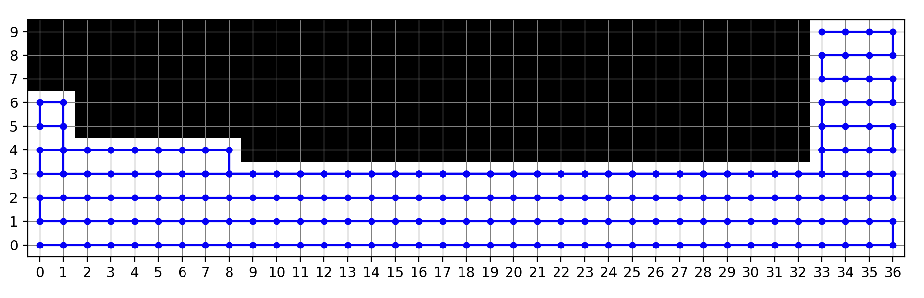
The CPP algorithm is the default but when an obstacle is encountered, it falls back to a-star to go around it before continuing with CPP. All free squares are covered with no incursion into the blocked obstacles. This is the algorithm I will use to control the robot. It uses a function "is_obstacle_detected()" which checks the map for obstacles. This can be augmented later with sensor detection. i.e:

if map_obstacle_detected or sensor_obstacle_detected:
  return True
return False

Transferred to kupePi ok.

May 2026